
|
|
|
|
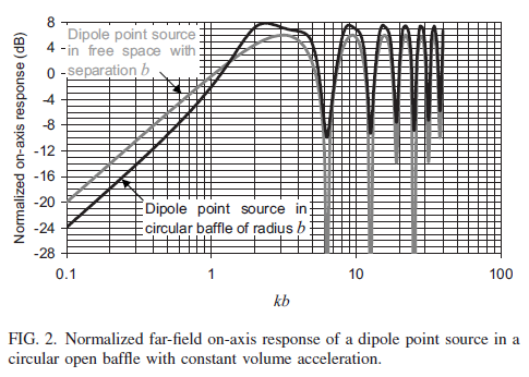 |
Figure 2 gives a
comparison of the on-axis response of a dipole point source in a
circular baffle to the on-axis response of a spaced dipole point source
as in A above [1].
Of particular interest to me is the change in low
frequency slope from 6 dB/oct to about 9 dB/oct before the response
levels out. The change in slope is due to baffle edge diffraction. I
have observed such change in slope in all my dipole designs and had
assumed it was due to driver asymmetry. The behavior makes equalization
for a flat response more difficult. A notch filter is required in
addition to the low frequency boost at 6 dB/oct rate in order to turn
the corner to a flat acoustic response. kb = 2p(b/l) |
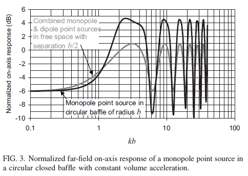 |
Figure 3 shows
corresponding behavior of a monopole point source in a circular, flat
baffle due to edge diffraction [1].
The response is different from what popular edge diffraction models show for this case (light gray curve). It is commonly referred to as "baffle step". I have observed poor correlation between predicted on-axis frequency response from such multi-point-source edge diffraction models and actual acoustic measurements. |
[1] Tim Mellow & Leo Karkkainen, "A dipole loudspeaker with balanced directivity pattern", J. Acoust. Soc. Am. 128 (5), November 2010, pp. 2749 - 2757
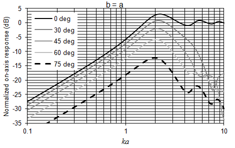
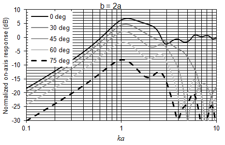
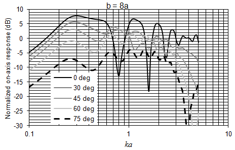
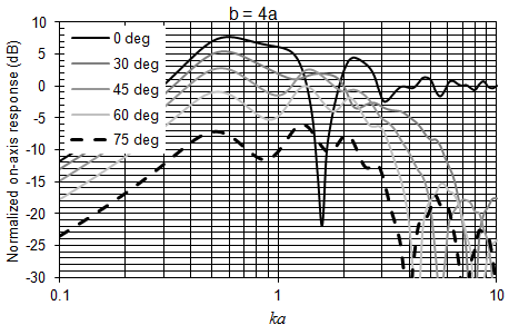
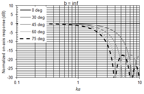
The normalized on-axis response of a plane circular piston of radius a in a flat open circular baffle of radius b was calculated by Tim Mellow for b = a, 2a, 4a, 8a, inf., and also polar responses were plotted in: Leo L. Beranek & Tim J. Mellow, Acoustics - Sound Fields and Transducers, Elsevier (2012), Chapter 13 - Radiation and scattering of sound by the boundary integral solution. It is instructive to see how the calculated responses differ from those predicted by the simple point source and edge diffraction models used here and elsewhere. In particular, the change in slope to >6 dB/oct just below the dipole peak and reduced ripple in the response above the peak confirm experimental observations.
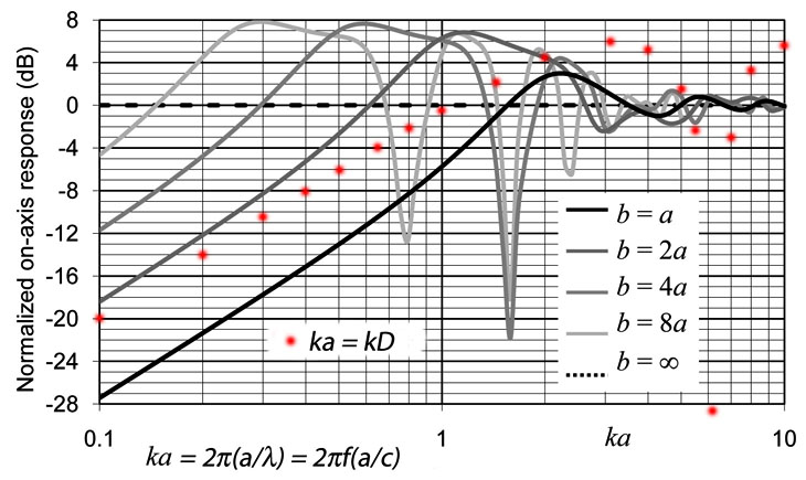
A3-1 Normalized on-axis response of a
plane circular piston of radius a in a flat open circular baffle of
radius b. |
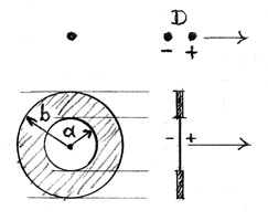
A3-2 Plane circular piston of radius
a in a flat open baffle of radius b (bottom). |
The on-axis response for the point source model deviates significantly from the response of the circular piston (A3-2). The slope is greater than -6 dB below the dipole peak for the piston (A3-1). This is in agreement with the typically required dipole equalization. Above the dipole peak the ripple is minimal for the unbaffled piston. This was also confirmed in the development of the LX521 midrange baffle shape.
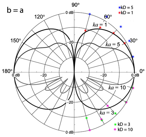
A3-3 Far-field radiation pattern for
a plane circular piston of radius a radiating from both sides into free
space without a baffle as a function of ka. |
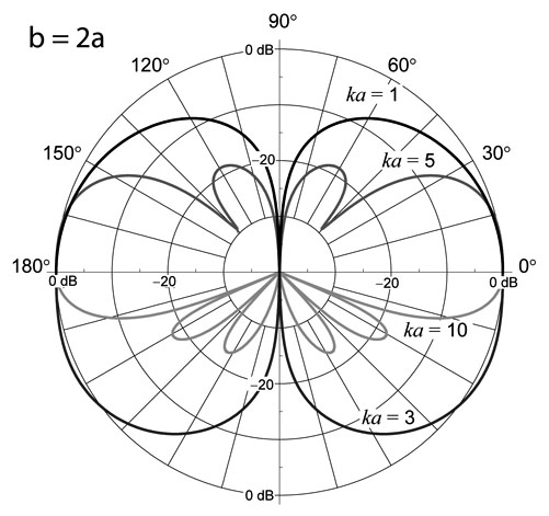
A3-4 Far-field radiation pattern for
a plane circular piston of radius a in a flat circular baffle of radius
2a radiating from both sides into free space as a function of ka. |
The radiation pattern of the point source model agrees with the unbaffled circular piston only for kD << 1, at long wavelengths and low frequencies where it follows a cos(alpha) pattern (A3-3). In general the pattern of the point sources is wider at higher frequencies as seen for kD = 3, 5, 10, while the piston starts to narrow its pattern. The two point source model is not a realistic guide to understanding practical dipole behavior for kD > 1. When a baffle is added to the piston then the pattern narrows even further and more side lobes and interference notches are created (A3-4). Adjacent lobes have opposite polarity.
 |
A3-5 The data are presented as frequency normalized on- and off-axis response curves for different radius of the flat baffle. I thank Tim Mellow and Leo Karkkainen for generating the graphs, which required many hours of computer time. The graph for b=8a had to be truncated at ka = 5 because each data point took hours to calculate. The curves approach the infinite case. Leo is still experimenting with ways to speed up
the calculations for a piston in an open rectangular baffle of specified
aspect ratio, which turns the analysis into a 3-dimensional problem.
They have derived exact formulas, but the computational effort is
immense. |
 |
 |
 |
 |
See also Figure 5 to Figure 7 in the paper by Tim Mellow & Leo Karkkainen, "On the
sound field of an oscillating disk in a finite open and closed circular
baffle".
Top
There is not much sense in building a dipole speaker with two small closed box speakers driven in opposite phase, when one of the objectives is to remove the sound character that boxes impart. The two boxes a can be joined at their backs, though, and the connecting wall removed b.

Since the two cones move back and forth in unison, there
is little air pressure inside the enclosure b at very low frequencies.
When the internal length L becomes half wavelength,
there is a sharp resonance of the transmission line between the cones, causing a
severe dip and peak irregularity in the frequency response. The two drivers in b
can be replaced by a single driver c without loss in volume displacement
capability. The latter arrangement, called H baffle, is very practical for
dipole woofer construction. It too has a severe resonance because the waveguide
of effective length L in front and behind the cone sees large impedance
mismatches at the cone and at the open end of the cabinet. The resonance occurs
when L = l/4 =
0.25*v/F.
For a baffle of D = 20" (0.5 m) length and with L = 10" (0.25 m)
estimated, the resonance peak in the dipole output is at F = 0.25*v/L = 343 Hz.
Even when the peak is removed by equalization, the H baffle should only be
operated below this frequency. It is a compact baffle for woofer applications
and I use it with slightly different driver arrangement for the PHOENIX.
Output equal to a closed box occurs at Fequal = 0.17*v/D = 117 Hz with the 20"
path difference D between the positive and negative polarity sources at the H
baffle openings.
For a deeper analysis of the H-frame see the Issues in
speaker design page.
 Brian Elliott, November 2010 |
I saw the H-baffle concept for the first time, constructed as two woofer towers with six 12" drivers each, with D=16", and placed against the side walls, at the home of Brian J. Elliott, Ph.D, Consultant in Electro-Acoustics, in Palo Alto, 1988. I had never heard bass reproduced so naturally before. In 1989 we talked about dipole loudspeakers and reduced room interaction to the local AES group. Brian has designed and built some truly outstanding sound reproduction systems for extremely wealthy clients, though he hardly got rich in the process. He is too much of a researcher and scientist at heart. Later on, Don Barringer successfully experimented with a smaller version of the H-baffle and since then I have used variations of it in many of my designs. |
The closed dipole baffle b with two drivers can be evolved d into the flat, circular, open baffle e with a single driver, while maintaining the same excursion limited output capability.
The circular baffle with a -|+ point source at its center has nearly the same polar radiation pattern as the two opposite polarity point sources spaced D apart in the model of figure A1 above. The circular baffle's usefulness at high frequencies is limited by the sharp interference nulls when D is a multiple of a wavelength. This behavior can be considerably smoothed by making the baffle f rectangular which gives a variation to the length of D.
For structural and aesthetic reasons you may want to fold
back the baffle g. The baffle depth d must be kept shallow to avoid
forming a cavity which stores acoustic energy and resonates. The exact shape of
the folded baffle is best determined experimentally. Since there are no
significant forces on the baffle you can quickly construct it from heavy
corrugated card board. Only the drivers need to be held solidly in place.
Measure on-axis and off-axis frequency response as you vary width height and
depth.
This type of baffle can give you smoother response at all angles than is
possible with a closed box, because the rear radiation coming around to the
front can be used to advantage. With a closed box you only have the option to
make the baffle either very narrow or very wide for smooth horizontal
dispersion. For a discussion of diffraction and how it relates to open
baffles look at FAQ8.
As frequency increases and the driver becomes more directional of its own, the
polar pattern still has an approximately cos(a) shape, because the driver
radiates front and rear and little to the sides of the open baffle. Top
Completely open driver arrangements have been used by Celestion and Legacy
Audio. A simple model to describe this case would be given by two drivers mounted on their own small
baffles of effective radius d1 and separated by
2d2 from each other.
The model predicts that the SPL at very low frequencies is merely the sum of two dipoles with spacing D = d1. The separation 2d2 between them has no influence on the total output as long as it is small compared to the wavelength of radiation. I see no compounding effect other than summing two dipoles, but the two baffles might as well be placed next to each other. A single driver in an H-frame would have the same output if the distance D between the openings is 2d1. Even order non-linear distortion can be reduced by reversing one of the drivers in the compound configuration so that the two magnets face each other. The whole arrangement does not strike me as a very effective use of a second driver and cabinet space compared to an H or W frame. I have no data how high in frequency the "compound woofer" can be used, but its radiation pattern will become more lobing than that of the two point source woofer. Top
If you have build an H baffle woofer, then the first step is to measure the frequency response of the drivers in the cabinet, In general, you can expect that the air loading on the cones will reduce the mechanical resonance frequency Fs and increase Qt. There will also be a response peak due to a l/4 resonance of the waveguides in front and behind the drivers. The measurement is performed right at the opening of the cabinet, so that the microphone sees only one of the two sources that form the dipole. Therefore you will not see the characteristic 6 dB/oct dipole slope in the data.
The PHOENIX woofer has D=19" (0.48 m) separation between its openings. The peak should be at f = 0.5*v/D = 357 Hz, but the cabinet layout is too complicated for such simple calculation to apply exactly. The woofer will be crossed over at 100 Hz with a 12 dB/oct L-R low-pass filter. The resonance peak will not be attenuated sufficiently by the low-pass and must be removed first with a notch filter. This usually takes some trial and error to find the best trade-off. Top
From the graph, the 270 Hz peak rises about 11 dB. This requires the notch to dip down to -11 dB or to a = 10^(-11/20) = 0.28. The Q of the peak is about (270 Hz)/(100 Hz) = 2.7 and determines the width of the notch.
Select R1 = 5.11k, then R = 5110*0.28/(1-0.28) = 1987 ohm.
L = 2.7*1987/(2*pi*270) = 3.16 H and
C = 1/(3.16*(2*pi*270)^2) = 110 nF
The input impedance R2 of the following stage is assumed to be large, so that R2
can be neglected for the filter calculation.
The large size inductor L is best realized with an active circuit inductr2.gif.
The inductive reactance is X = 2*pi*270*3.16 = 5360 ohm. For
the inductor to have a Q of at least ten times the Q of the notch, the parallel
resistor must be greater than Rp = 10*2.7*5360 = 145 kohm. Select 147k as
standard value.
Rs needs to be smaller than R (1987 ohm). Select Rs = 511 ohm to give some
adjustment room for R.
Now find C = 3.16/(511*(147000-511)) = 42.2 nF.
Finally, reduce R because the inductor contributes already 511 ohm. R = 1987-511
= 1476 ohm.
Next step is to build a circuit with these values, insert it ahead of the power
amplifier and measure the woofer response to see if the peak has been removed to
your satisfaction or if the circuit values need further trimming.
The 290NF
stage in the PHOENIX crossover/eq
woofer channel has the final values and you can see that I had to do some
experimentation with R, L and C to obtain the equalized response in the graph above. It
also helps to use a SPICE based circuit analysis program for the notch filter
circuit to find the inverse of the peak response more readily than via the
approximate calculations above. Top
This part of the equalization is easy and only involves the decision at
which frequency to start and to end. A circuit that is suitable for the task is
the shelving low-pass. The woofer
dipole with D=19" has its first peak ideally at 357 Hz and transitions into
the 6 dB/oct slope somewhat below this frequency. Thus I chose f2 = 300 Hz. From
the measured woofer response above, you can see that it is quite flat and 3 dB
down at 13 Hz. Extending the equalization down to f1 = 10 Hz makes for a gradual
transition into the ultimately 18 dB/oct roll-off region of the dipole below the
driver resonance.
With those values we calculate from f2/f1 = 1+R2/R1 that
R2 = R1*((f2/f1) -1) = R1*((300/10)-1) = 29*R1.
Select R1 = 4.64k, then R2 = 134.6k or 133k as closest standard value.
Calculate C = 1/(2*pi*f1*R2) = 1/( 2*pi*10*133000) = 120 nF.
Check that f2 is indeed close to 300 Hz for the chosen values.
The circuit has a dc gain of 1+133/4.64 or 29.4 dB, which is high. This stage
should come after the level setting circuit to avoid clipping distortion.
The woofer equalization is now complete (x1.gif).
Top
You may be using a woofer which rolls off over a wider frequency range than
the one in the PHOENIX because its Qt in the cabinet is less than 0.7, or the
resonance frequency Fs is too high. In such cases you can equalize what you have
into a more desirable response by using a special biquad circuit f0Q0fpQp.gif.
To apply the circuit you must determine f0 and Q0 for the drivers in the cabinet
from a measurement of their terminal impedance according to f0Q0.gif.
Keep in mind that with the biquad you are setting the two complex poles of a 3rd
order high-pass filter. The 3rd, real axis pole is created by selecting f1
for the dipole slope correction. There is no transient optimum high-pass filter
like the Bessel filter for the low-pass case. The 3rd order Butterworth
high-pass has no other merits than to look pretty. Optimum for time response is
to place all three poles on the real axis, i.e. Qt = 0.5 for the dual poles, and
then the frequency response is 9 dB down at Fs. Better
yet, drivers with very low Qts < 0.5 make it possible to place two real
axis poles at 20 Hz and the 3rd pole around 5 Hz, but require more elaborate
equalization, because they roll off with a pole around 80 Hz in addition
to the 6 dB/oct dipole roll-off..
In general, I prefer the more gradual roll-off for any woofer, because it
corresponds to a more linear phase response (more uniform group delay) and that
is audible. The trade-off is in low end extension. Top
When you place a driver (e.g. SS 21W/8554) on a circular
open baffle, then you measure a response that differs somewhat from the model under
A.
At low frequencies the response follows the 6 dB/oct slope, but the first peak
and null are not clearly formed. Also, in the rear of the baffle, the response
rolls off more than in front.
Very important to note is the first response peak. It is a function of the driver used and almost all drivers exhibit it to varying degrees. The peak is caused by an acoustic filter formed by the basket openings and trapped air between cone and basket. This filter is the reason for the differences in high frequency response between front and rear.
A driver becomes directional of its own, when its effective piston diameter becomes larger than 1/3 of a wavelength. For an 8" driver this would be above 558 Hz. Still, the expected +6 dB dipole peak, when the rear wave adds fully to the front radiation at 838 Hz for the D = 8" circular baffle, can be seen in the measured data above. The expected null at 1675 Hz, though, is only partially formed, because not enough energy comes around the baffle edge.
The combined response of the two 8" drivers mounted on the PHOENIX baffle also exhibits a peak due to the basket resonators. The peak must first be removed with a notch-filter, so that a shelving low-pass filter equalization can give the proper transition from the 6 dB/oct region into the flat region of the dipole response.
The off-axis response at 30, 45 and 60 degrees exhibits
some interesting characteristics. At low frequencies it follows the cos(a)
pattern as in the dipole model under A above. Around 700 Hz and 1500 Hz the
horizontal pattern actually widens, and only above 2 kHz becomes the pattern
progressively narrower, as indicated by the separation of the response curves
for different angles. The pattern would become narrow at much lower frequency,
if you closed the back of the baffle.
The vertical polar response is
dominated by the separation of the 8" drivers and therefore much narrower.
On and off-axis response are very much a function of baffle shape and the amount
of fold-back. Computer models are not available and the optimum shape must be
determined experimentally.
With the above as background in mind, the midrange dipole
equalization follows the steps outlined for the woofer under C. The only
difference is the choice of frequency f1 for the shelving
low-pass. Since the chosen crossover to the PHOENIX woofer is of 2nd-order,
one of the two 1st-order high-pass sections can be realized by placing f1 at the
crossover frequency of 100 Hz. The second high-pass filter is realized with the
90HP stage of the crossover/eq.
It is easiest to model the equalizer with a circuit CAD program and to compare
response curves to the measured data. The low Q of the notch filter (x1.gif)
makes it
difficult to predict circuit values with sufficient accuracy and requires
iteration. Top
We start the crossover design with on-axis and horizontal off-axis frequency response measurements of the tweeter and the two midrange drivers on the PHOENIX main panel. It is important to know the off-axis behavior in order to choose the crossover frequency such that the combined midrange and tweeter response is as smooth as possible off-axis. The on axis ripples in the tweeter response are a mixture of diffraction off the midrange driver cones in the M-T-M arrangement, primarily at lower frequencies, and diffraction off the panel edges at higher frequencies. No attempt has been made to further reduce these effects by equalization, because they are dominant only on-axis and smoothed out off-axis.
The drivers have a 13 dB difference in sensitivity. The
midrange channel gain will be set 13 dB lower than the tweeter channel to
correct for this (x1.gif).
Selecting a 1400 Hz crossover frequency based on dispersion gives wide overlap
between the drivers. The tweeter goes almost 2 octaves lower and the midrange 2
octaves higher with useable flatness. Thus, when a 24 dB/oct L-R
electrical crossover filter at 1400 Hz is used, the combined driver
and filter magnitude (dB) response will be mainly that of the electrical
circuit. This specific situation reduces the design of the desired 24 dB/oct L-R
acoustical crossover to the selection of components for a well known electrical
circuit. Standard component values result in 1440 Hz high-pass filters in the
tweeter channel and 1440 Hz low-pass filters in the midrange channel of the crossover/eq.
The crossover frequency at 1400 Hz is quite low and
therefore it is important to assure that the tweeter has adequately low
distortion at the volume displacements required.
From the SS D2905/9700 specification of Xmax = 0.5 mm linear and 8.5 cm^2 cone
area you estimate an SPL = 101 dB at 1400 Hz, 1 m,
free space, closed box. Add to this 6 dB lift from the baffle and 6 dB from the midrange
contribution for a total of 113 dB SPL. Maximum displacement is 1.5 mm or 10 dB
higher. The tweeter is within the desired range, but harmonic distortion,
intermodulation distortion, stored energy measurements and listening tests must
be additional criteria for choosing it.
The crossover design is not complete yet, because the
tweeter's high-pass behavior and the midrange's roll-off cause phase shifts that
are part of the crossover. In addition, the physical offset between driver voice
coils causes delays and associated phase shift that must be corrected. This is
best done experimentally and started with the driver offset.
The tweeter is approximately 2" (0.05 m) in front of the midranges and its
input signal must be delayed by T = d/v = 0.05/343 = 146 us to be in phase with
the midranges. The group delay of an all-pass
circuit is used for the offset compensation.
The delay of the circuit changes with frequency, but the
1400 Hz crossover should fall into the flat region of the delay and therefore f0
> 1400 Hz. You can estimate the number of stages required from this
inequality.
If f0 = 1/(2*pi*R*C) > 1400 and thus
R*C < 1/(2*pi*1400) = 114 us,
then a single stage would have to be operated in its sloping region to obtain
146 us of delay. Thus take two stages. The actual implementation in the tweeter
channel provides 85 us and 104 us for a total of 189 us. The value is larger
than estimated, because the low-pass behavior of the midranges moves their voice
coils effectively further behind the tweeter than the physical distance
measurement.
The final component values for the all-pass circuits have been determined
experimentally from an optimization of the combined midrange and tweeter frequency
response. The depth of the interference notch when the tweeter polarity is
reversed, is an indication of how closely the two outputs are to being 180
degrees out-of-phase and of equal magnitude. Top
From C above you can see that the dipole woofer's useable frequency range after equalization extends to 250 Hz at the most. If the response should follow the crossover low-pass filter closely over the first octave of roll-off, then the crossover frequency cannot be higher than 100 Hz.
Initially, I used a 24 dB/oct L-R crossover for a similar speaker, the Audio Artistry Dvorak, but we found after extensive listening that a 12 dB/oct L-R gave a slight improvement in bass realism. I think this is due to the more gradual transition of the group delay response of the 1st order all-pass formed by the lower order crossover vs. the 2nd order all-pass for the 24 dB/oct crossover. I had found earlier (Ref. 17) that phase distortion is audible at low frequencies even with a 1st order allpass. At high frequencies it must be much more severe than the phase distortion of a 24 dB/oct L-R crossover before it becomes audible.
I have recently investigated my previous assumption about the audibility of reduced phase distortion from a 12 dB/oct crossover between woofer and midrange, with the conclusion that the difference in phase shift between a 12 dB/oct and a 24 dB/oct crossover is not audible, not even when compared to a zero distortion 6 dB/oct crossover. Thus it would seem reasonable to use the higher order crossover which reduces the potential for non-linear distortion in the midrange driver and attenuates any higher frequency contribution from the woofer. I invite anyone interested to test for themselves the validity of my observation.
A 12 dB/oct crossover places much greater demands on the excursion capability of the midrange drivers. When you apply a constant voltage to the driver terminals, then the cone excursion X1 increases at a 12 dB/oct rate going down in frequency, figure a. Below the driver resonance Fs the excursion X1 becomes constant. Dipole equalization Veq boosts the excursion at +6 dB/oct up to the crossover frequency Fxo to give a flat SPL response. The terminal voltage decreases at 6 dB/oct rate below Fxo and, in conjunction with the dipole roll-off of 6 dB/oct, gives the 12 dB/oct acoustic high-pass filter response for the L-R crossover.
The net effect of equalization for flat response and of the 12 dB/oct crossover is an increase of excursion X2 at 18 dB/oct above Fxo, 6 dB/oct below it, and a decrease at 6 dB/oct below Fs as in figure b.
The SS 21W/8554 8" driver on the PHOENIX main panel
has 200 cm^2 piston area, 6.5 mm linear excursion and 10 mm Xmax. With an
effective back to front path length D of 9.75" (248 mm) the dipole SPL at
100 Hz, 1 m, becomes 97 dB. The second driver
increases the value by 6 dB and the woofer contributes another 6 dB for a total
of 109 dB SPL. Driven to Xmax adds 4 dB more.
Note, that If you wanted to maintain 113 dB SPL down to 25 Hz, then the
displacement of the two 8" drivers would have to increase another 12 dB (X2
figure b) to 4*10 mm = 40 mm peak, even though its contribution to the
total SPL output would be 24 dB below the woofer output. In reality the 8"
drivers can maximally support 113 -12 = 101 dB SPL at 25 Hz.
You can begin to see why I added two 10" drivers to the AA Beethoven and four 10" drivers to the Beethoven-Grand to cover the range below 200 Hz. The transition between 10" and 8" drivers is at 6 dB/oct for group delay reasons, but requires phase compensation to steer the vertical polar pattern towards the listener. Such 4-way system is a little tricky to design and measure.
The 12 dB/oct 100 Hz crossover for two 8" drivers is thus a trade-off between maximum sound level and sound quality. Circuit implementation is straight forward with a 2nd order low-pass (99LP) in the woofer channel, the midrange dipole boost ending at 100 Hz (90-500LP) and a 100 Hz high-pass filter (90HP) in the midrange channel. The actual filter corner frequencies differ from the nominal values due to standard component value selection and trimming of the measured crossover response (x1.gif). Top
The crossover is not complete without setting the proper woofer level relative to the midrange. It is difficult to set by listening to program material because recordings vary greatly and room resonances can change the perceived level. It is best to start with outdoor measurements and to refine the result by indoor listening if a technically justifiable reason exists for it. (I am assuming that you want to build a transducer and not a musical instrument)
For the outdoor measurement you might might raise woofer and main panel some large distance Y above ground to minimize and delay the effect of reflections, figure a. Assume you adjust the system to be flat through the crossover region and beyond. Now, when you set the woofer on the ground and the panel at normal listening height, figure b, the woofer output will receive a uniform 6 dB boost because it radiates into half-space.
The output from the panel will not increase 6 dB except at
low frequencies where the sounds via the direct ray and the ground reflected ray
to the listener L are almost in phase. At higher frequencies the ground
reflection subtracts and adds periodically. The panel essentially radiates into
full-space as in figure a, but with floor reflection superimposed to the
response at L. If we left the woofer level adjustment as found in a, then
the woofer contribution at the listening position in b would be 6 dB too
high relative to the high frequencies from the panel. At low frequencies the
panel receives a similar ground boost and its output becomes too large relative
to its high frequencies.
The transition region between full-space and half-space radiation is equalized
with a shelving high-pass filter that
gives a 6 dB cut to very low frequencies and has a gradual transition with
corner frequencies at 100 Hz and 200 Hz. I determined the frequency values
empirically. The filter (100-200HP)
is placed ahead of midrange and woofer channels to affect both (x1.gif).
Instead of measuring the combined frequency response at large elevation as in figure a, I measure it with the microphone on the ground, figure b. Under these conditions woofer and panel receive the same ground boost and no shelving filter is used. Crossover filters are trimmed and woofer level set for flat response. In my case this is not a completely reflection free measurement because of adjacent buildings and structures and I use some mental averaging of the wiggles. Ambient noise tends to limit the low frequency dynamic range and I therefore pre-emphasize the low frequencies of the MLS stimulus signal to increase measurement range.
When I now measure at L in figure b I find that the low frequency response is too high, but correct when the shelving filter is in the circuit.
Unfiltered and octave smoothed curves are shown above.
We usually do not listen outdoors, but even in a room we have the same floor effects. In addition there are the effects due to modes, if excited, and they become superimposed to the above response and should be dealt with separately, for example by room equalization with notch filters. The PHOENIX printed circuit board provides layouts for this. Top
The gain of the midrange channel is held constant. Tweeter and woofer outputs are adjusted relative to it. Since the midrange driver voltage sensitivity is 12 dB higher than the tweeter (see E above) I use a 12 dB attenuator ahead of the dipole equalization (90-500LP). The 400NF notch filter, which is driven from the attenuator, must see an impedance of 5k ohm for proper equalization of the midrange peak as determined by experiment. Thus it becomes necessary to design a resistive ladder with an attenuation factor a = 10^(-12/20) = 0.25 and 5000 ohm output impedance.
For the variable gain in the woofer and tweeter channel I chose a 5 dB adjustment range which also matches with the10 tick marks on the trim potentiometer. The linear dB scale is generated with a circuit that I saw used by my former colleague Russ Riley. I have found many applications for it.
R4 is a linear 1k ohm potentiometer. The values for R3 and
R5 are determined from gmax = 0 dB (1.0) and gmin = -5 dB (0.56) with a little
algebra as R3 = 3.55k and R5 = 2.55k. The closest standard series values of
3.48k and 2.61k are used for the tweeter channel gain adjustment.
The woofer channel requires about 8 dB (0.40) of attenuation to match up with
the midrange. A resistive ladder is used for this with an output impedance
target Rout = R3 = 3.55k ohm to drive the variable gain stage (+/-2.5
dB). Top
Our perception of loudness is slightly different for
sounds arriving frontally versus sounds arriving from random directions at our
ears. The difference between equal-loudness-level contours in frontal
free-fields and diffuse sound fields is documented, for example, in ISO
Recommendation 454 and in E. Zwicker, H. Fastl, Psycho-acoustics, p. 205.
Diffuse field equalization of dummy-head recordings is
discussed in J. Blauert, Spatial Hearing, pp. 363, and headphone diffuse field equalization by
G. Theile in JAES, Vol. 34, No. 12.
Reference to a slight dip in the 1 to 3 kHz region for loudspeaker equalization
is made in H. D. Harwood (BBC Research Department), Some factors in loudspeaker
quality, Wireless World, May 1976, p.48.
Around 3 kHz our hearing is less sensitive to diffuse
fields. Recording microphones, though, are usually flat in frequency response
even under diffuse field conditions. When such recordings are played back over
loudspeakers, there is more energy in the 3 kHz region than we would have
perceived if present at the recording venue and a degree of unnaturalness is
introduced.
This applies primarily to recordings of large orchestral pieces in concert halls
where the microphones are much closer to the instruments than any listener. At
most listening positions in the hall the sound field has strong diffuse
components.
I use a dip of 4 dB (x1.gif, 2760NF)
to equalize for this. The circuit consists of R, C and L in series, forming a
frequency dependent ladder attenuator in conjunction with the 5.11k ohm source
resistor. You may choose to make the notch filter selectable with a switch
for different types of recordings.
I have found through my own head-related recordings of symphonic music that the dip adds greater realism, especially to large chorus and to soprano voice and allows for higher playback levels. Top
Normally the equivalent 1 m sound pressure level of a speaker is specified for a 2.83 V signal at the crossover input terminals. This would correspond to 1 W into 8 ohm if the terminal impedance was actually 8 ohm. Defining the 2.83 V, 1 m sensitivity for a system with electronic crossover/eq like the PHOENIX is not as straight forward.
Starting with the SS D2904/9800 tweeter, the
manufacturer's specification is 90 dB SPL, 2.83 V, 1 m.
Sensitivity of the two midranges, wired in parallel, and mounted in the open
baffle measures about 13 dB higher
than the tweeter or 103 dB SPL. The SS specification is 90 dB SPL for a single
21W/8554 driver. For two drivers in parallel add 6 dB and for rear radiation
reinforcement from the open baffle add another 6 dB, which explains the high
measured value. The crossover circuit attenuates the signal to the midrange
power amplifier by 13 dB except towards the lower frequencies where the 6 dB/oct
dipole equalization and the crossover roll-off come in. The 7
dB boost at 100 Hz makes up for the loss in midrange sensitivity from 103 dB
above 250 Hz to 103 - 7 = 96 dB SPL at 100 Hz.
The 1252DVC woofer driver has a 91 dB SPL specification which applies at Fequal
= 0.17*v/D = 121 Hz. With two drivers in parallel the sensitivity becomes 97 dB,
but rolls off at 6 dB/oct rate below 121 Hz. Thus at 60 Hz the sensitivity is 91
dB SPL and goes down to 85 dB SPL at 30 Hz.
The above SPL values are for 2.83 V across the driver terminals. With a tweeter impedance of about 4.5 ohm over its used frequency range this corresponds to (2.83)^2 / 4.5 = 1.8 W. For the paralleled midranges with 3.5 ohm impedance the power becomes 2.3 W and <1.2 W for the woofer drivers at >6.5 ohm total.
For an estimate of the power required to obtain a desired SPL level in an enclosed space at listening position see the discussion of "Room reverberation time T60" on the Room acoustics page. Top
-------------------------------
The Frequently Asked Questions page will show you answers to inquiries which I received about the PHOENIX project and related subjects.
| Build-Your-Own | Main Panel
| Dipole Woofer | Crossover/EQ
| Supplies |
| System Test | Design
Models | Prototypes | Active
Filters | Surround | FAQ
|
|
| ||||

